4. The Kolmogorov Backward Equation#
In addition to what’s in Anaconda, this lecture will need the following libraries:
!pip install quantecon
4.1. Overview#
As models become more complex, deriving analytical representations of the Markov semigroup \((P_t)\) becomes harder.
This is analogous to the idea that solutions to continuous time models often lack analytical solutions.
For example, when studying deterministic paths in continuous time, infinitesimal descriptions (ODEs and PDEs) are often more intuitive and easier to write down than the associated solutions.
(This is one of the shining insights of mathematics, beginning with the work of great scientists such as Isaac Newton.)
We will see in this lecture that the same is true for continuous time Markov chains.
To help us focus on intuition in this lecture, rather than technicalities, the state space is assumed to be finite, with \(|S|=n\).
Later we will investigate the case where \(|S| = \infty\).
We will use the following imports
import numpy as np
import scipy as sp
import matplotlib.pyplot as plt
import quantecon as qe
from numba import njit

from scipy.linalg import expm
from scipy.stats import binom
4.2. State Dependent Jump Intensities#
As we have seen, continuous time Markov chains jump between states, and hence can have the form
where \((J_k)\) are jump times and \((Y_k)\) are the states at each jump.
(We are assuming that \(J_k \to \infty\) with probability one, so that \(X_t\) is well defined for all \(t \geq 0\), but this is always true for when holding times are exponential and the state space is finite.)
In the previous lecture,
the sequence \((Y_k)\) was drawn from a Markov matrix \(K\) and called the embedded jump chain, while
the holding times \(W_k := J_k - J_{k-1}\) were IID and Exp\((\lambda)\) for some constant jump intensity \(\lambda\).
In this lecture, we will generalize by allowing the jump intensity to vary with the state.
This difference sounds minor but in fact it will allow us to reach full generality in our description of continuous time Markov chains, as clarified below.
4.2.1. Motivation#
As a motivating example, recall the inventory model, where we assumed that the wait time for the next customer was equal to the wait time for new inventory.
This assumption was made purely for convenience and seems unlikely to hold true.
When we relax it, the jump intensities depend on the state.
4.2.2. Jump Chain Algorithm#
We start with three primitives
An initial condition \(\psi\),
a Markov matrix \(K\) on \(S\) satisfying \(K(x, x) = 0\) for all \(x \in S\) and
a function \(\lambda\) mapping \(S\) to \((0, \infty)\).
The process \((X_t)\)
starts at state \(x\), draw from \(\psi\),
waits there for an exponential time \(W\) with rate \(\lambda(x)\) and then
updates to a new state \(y\) drawn from \(K(x, \cdot)\).
Now we take \(y\) as the new state for the process and repeat.
Here is the same algorithm written more explicitly:
Algorithm 4.1 (Jump Chain Algorithm)
Inputs \(\psi \in \dD\), rate function \(\lambda\), Markov matrix \(K\)
Outputs Markov chain \((X_t)\)
Draw \(Y_0\) from \(\psi\), set \(J_0 = 0\) and \(k=1\).
Draw \(W_k\) independently from Exp\((\lambda(Y_{k-1}))\).
Set \(J_k = J_{k-1} + W_k\).
Set \(X_t = Y_{k-1}\) for \(t\) in \([J_{k-1}, J_k)\).
Draw \(Y_k\) from \(K(Y_{k-1}, \cdot)\).
Set \(k = k+1\) and go to step 2.
The sequence \((W_k)\) is drawn as an IID sequence and \((W_k)\) and \((Y_k)\) are drawn independently.
The restriction \(K(x,x) = 0\) for all \(x\) implies that \((X_t)\) actually jumps at each jump time.
4.3. Computing the Semigroup#
For the jump process \((X_t)\) with time varying intensities described in the jump chain algorithm, calculating the Markov semigroup is not a trivial exercise.
The approach we adopt is
Use probabilistic reasoning to obtain an integral equation that the semigroup must satisfy.
Convert the integral equation into a differential equation that is easier to work with.
Solve this differential equation to obtain the Markov semigroup \((P_t)\).
The differential equation in question has a special name: the Kolmogorov backward equation.
4.3.1. An Integral Equation#
Here is the first step in the sequence listed above.
Lemma 4.1 (An Integral Equation)
The semigroup \((P_t)\) of the jump chain with rate function \(\lambda\) and Markov matrix \(K\) obeys the integral equation
for all \(t \geq 0\) and \(x, y\) in \(S\).
Here \((P_t)\) is the Markov semigroup of \((X_t)\), the process constructed via Algorithm 4.1, while \(K P_{t-\tau}\) is the matrix product of \(K\) and \(P_{t-\tau}\).
Proof. Conditioning implicitly on \(X_0 = x\), the semigroup \((P_t)\) must satisfy
Regarding the first term on the right hand side of (4.2), we have
where \(I(x, y) = \mathbb 1\{x = y\}\).
For the second term on the right hand side of (4.2), we have
Evaluating the expectation and using the independence of \(J_1\) and \(Y_1\), this becomes
4.3.2. Kolmogorov’s Differential Equation#
We have now confirmed that the semigroup \((P_t)\) associated with the jump chain process \((X_t)\) satisfies (4.1).
Equation (4.1) is important but we can simplify it further without losing information by taking the time derivative.
This leads to our main result for the lecture
Theorem 4.1 (Kolmogorov Backward Equation)
The semigroup \((P_t)\) of the jump chain with rate function \(\lambda\) and Markov matrix \(K\) satisfies the Kolmogorov backward equation
The derivative on the left hand side of (4.4) is taken element by element, with respect to \(t\), so that
The proof that differentiating (4.1) yields (4.4) is an important exercise (see below).
4.3.3. Exponential Solution#
The Kolmogorov backward equation is a matrix-valued differential equation.
Recall that, for a scalar differential equation \(y'_t = a y_t\) with constant \(a\) and initial condition \(y_0\), the solution is \(y_t = e^{ta} y_0\).
This, along with \(P_0 = I\), encourages us to guess that the solution to Kolmogorov’s backward equation (4.4) is
where the right hand side is the matrix exponential, with definition
Working element by element, it is not difficult to confirm that the derivative of the exponential function \(t \mapsto e^{tQ}\) is
Hence, differentiating (4.5) gives \(P'_t = Q e^{t Q} = Q P_t\), which convinces us that the exponential solution satisfies (4.4).
Notice that our solution
for the semigroup of the jump process \((X_t)\) associated with the jump matrix \(K\) and the jump intensity function \(\lambda \colon S \to (0, \infty)\) is consistent with our earlier result.
In particular, we showed that, for the model with constant jump intensity \(\lambda\), we have \(P_t = e^{t \lambda (K - I)}\).
This is obviously a special case of (4.8).
4.4. Properties of the Solution#
Let’s investigate further the properties of the exponential solution.
4.4.1. Checking the Transition Semigroup Properties#
While we have confirmed that \(P_t = e^{t Q}\) solves the Kolmogorov backward equation, we still need to check that this solution is a Markov semigroup.
Lemma 4.2 (From Jump Chain to Semigroup)
Let \(\lambda\) map \(S\) to \(\RR_+\) and let \(K\) be a Markov matrix on \(S\). If \(P_t = e^{t Q}\) for all \(t \geq 0\), where \(Q(x, y) = \lambda(x) (K(x, y) - I(x, y))\), then \((P_t)\) is a Markov semigroup on \(S\).
Proof. Observe first that \(Q\) has zero row sums, since
As a small exercise, you can check that, with \(1\) representing a column vector of ones, the following is true
This implies that \(Q^k 1 = 0\) for all \(k\) and, as a result, for any \(t \geq 0\),
In other words, each \(P_t\) has unit row sums.
Next we check nonnegativity of all elements of \(P_t\) (which can easily fail for matrix exponentials).
To this end, adopting an argument from [Stroock, 2013], we set \(m := \max_x \lambda(x)\) and \(\hat P := I + Q / m\).
It is not difficult to check that \(\hat P\) is a Markov matrix and \(Q = m( \hat P - I)\).
Recalling that, for matrix exponentials, \(e^{A+B} = e^A e^B\) whenever \(AB = BA\), we have
It is clear from this representation that all entries of \(e^{tQ}\) are nonnegative.
Finally, we need to check the continuity condition \(P_t(x, y) \to I(x,y)\) as \(t \to 0\), which is also part of the definition of a Markov semigroup. This is immediate, in the present case, because the exponential function is continuous, and hence \(P_t = e^{tQ} \to e^0 = I\).
We can now be reassured that our solution to the Kolmogorov backward equation is indeed a Markov semigroup.
4.4.2. Uniqueness#
Might there be another, entirely different Markov semigroup that also satisfies the Kolmogorov backward equation?
The answer is no: linear ODEs in finite dimensional vector space with constant coefficients and fixed initial conditions (in this case \(P_0 = I\)) have unique solutions.
In fact it’s not hard to supply a proof — see the exercises.
4.5. Application: The Inventory Model#
Let us look at a modified version of the inventory model where jump intensities depend on the state.
In particular, the wait time for new inventory will now be exponential at rate \(\gamma\).
The arrival rate for customers will still be denoted by \(\lambda\) and allowed to differ from \(\gamma\).
For parameters we take
α = 0.6
λ = 0.5
γ = 0.1
b = 10
Our plan is to investigate the distribution \(\psi_T\) of \(X_T\) at \(T=30\).
We will do this by simulating many independent draws of \(X_T\) and histogramming them.
(In the exercises you are asked to calculate \(\psi_T\) a different way, via (4.8).)
@njit
def draw_X(T, X_0, max_iter=5000):
    """
    Generate one draw of X_T given X_0.
    """

    J, Y = 0, X_0
    m = 0

    while m < max_iter:
        s = 1/γ if Y == 0 else 1/λ
        W = np.random.exponential(scale=s)  # W ~ E(λ)
        J += W
        if J >= T:
            return Y
        # Otherwise update Y
        if Y == 0:
            Y = b
        else:
            U = np.random.geometric(α)
            Y = Y - min(Y, U)
        m += 1


@njit
def independent_draws(T=10, num_draws=100):
    "Generate a vector of independent draws of X_T."

    draws = np.empty(num_draws, dtype=np.int64)

    for i in range(num_draws):
        X_0 = np.random.binomial(b+1, 0.25)
        draws[i] = draw_X(T, X_0)

    return draws
T = 30
n = b + 1
draws = independent_draws(T, num_draws=100_000)
fig, ax = plt.subplots()

ax.bar(range(n), [np.mean(draws == i) for i in range(n)], width=0.8, alpha=0.6)
ax.set_xlabel("inventory", fontsize=14)

plt.show()
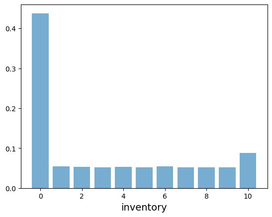
If you experiment with the code above, you will see that the large amount of mass on zero is due to the low arrival rate \(\gamma\) for inventory.
4.6. Exercises#
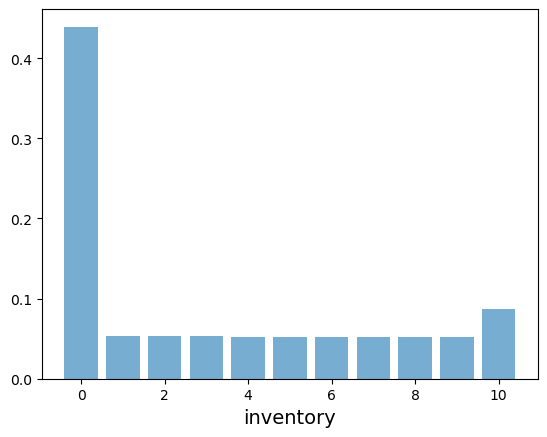
Exercise 4.1
In the discussion above, we generated an approximation of \(\psi_T\) when \(T=30\), the initial condition is Binomial\((n, 0.25)\) and parameters are set to
α = 0.6
λ = 0.5
γ = 0.1
b = 10
The calculation was done by simulating independent draws and histogramming.
Try to generate the same figure using (4.8) instead, modifying code from our lecture on the Markov property.
Solution
Here is one solution:
α = 0.6
λ = 0.5
γ = 0.1
b = 10

states = np.arange(n)
I = np.identity(n)

# Embedded jump chain matrix
K = np.zeros((n, n))
K[0, -1] = 1
for i in range(1, n):
    for j in range(0, i):
        if j == 0:
            K[i, j] = (1 - α)**(i-1)
        else:
            K[i, j] = α * (1 - α)**(i-j-1)

# Jump intensities as a function of the state
r = np.ones(n) * λ
r[0] = γ

# Q matrix
Q = np.empty_like(K)
for i in range(n):
    for j in range(n):
        Q[i, j] = r[i] * (K[i, j] - I[i, j])

def P_t(ψ, t):
    return ψ @ expm(t * Q)

ψ_0 = binom.pmf(states, n, 0.25)
ψ_T = P_t(ψ_0, T)

fig, ax = plt.subplots()

ax.bar(range(n), ψ_T, width=0.8, alpha=0.6)
ax.set_xlabel("inventory", fontsize=14)

plt.show()
Solution
One can easily verify that, when \(f\) is a differentiable function and \(\alpha > 0\), we have
Note also that, with the change of variable \(s = t - \tau\), we can rewrite (4.1) as
Applying (4.10) yields
After minor rearrangements this becomes
which is identical to (4.4).
Exercise 4.3
We claimed above that the solution \(P_t = e^{t Q}\) is the unique Markov semigroup satisfying the backward equation \(P'_t = Q P_t\).
Try to supply a proof.
(This is not an easy exercise but worth thinking about in any case.)
Solution
Here is one proof of uniqueness.
Suppose that \((\hat P_t)\) is another Markov semigroup satisfying \(P'_t = Q P_t\).
Fix \(t > 0\) and let \(V_s\) be defined by \(V_s = P_s \hat P_{t-s}\) for all \(s \geq 0\).
Note that \(V_0 = \hat P_t\) and \(V_t = P_t\).
Note also that \(s \mapsto V_s\) is differentiable, with derivative
where, in the second last equality, we used (4.7).
Hence \(V_s\) is constant, so our previous observations \(V_0 = \hat P_t\) and \(V_t = P_t\) now yield \(\hat P_t = P_t\).
Since \(t\) was arbitrary, the proof is now done.