1. Memoryless Distributions#
In addition to what’s in Anaconda, this lecture will need the following libraries:
!pip install quantecon
1.1. Overview#
Markov processes are, by definition, forgetful.
In particular, for any Markov processes, the distribution over future outcomes depends only on the current state, rather than the entire history.
In the case of continuous time Markov chains, which jump between discrete states, this requires that the amount of elapsed time since the last jump is not helpful in predicting the timing of the next jump.
In other words, the jump times are “memoryless”.
It is remarkable that the only distribution on \(\RR_+\) with this property is the exponential distribution.
Similarly, the only memoryless distribution on \(\ZZ_+\) is the geometric distribution.
This lecture tries to clarify these ideas.
We will use the following imports:
import numpy as np
import matplotlib.pyplot as plt
import quantecon as qe
from numba import njit
from scipy.special import factorial, binom
1.2. The Geometric Distribution#
Consider betting on a roulette wheel and suppose that red has come up four times in a row.
Since five reds in a row is an unlikely event, many people instinctively feel that black is more likely on the fifth spin — “Surely black will come up this time!”
But rational thought tells us such instincts are wrong: the four previous reds make no difference to the outcome of the next spin.
(Many casinos offer an unlimited supply of free alcoholic beverages in order to discourage this kind of rational analysis.)
A mathematical restatement of this phenomenon is: the geometric distribution is memoryless.
1.2.1. Memorylessness#
Let \(X\) be a random variable supported on the nonnegative integers \(\ZZ_+\).
We say that \(X\) is geometrically distributed if, for some \(\theta\) satisfying \(0 \leq \theta \leq 1\),
An example can be constructed from the discussion of the roulette wheel above.
Suppose that,
the outcome of each spin is either red or black,
spins are labeled by \(0, 1, 2, \ldots\),
on each spin, black occurs with probability \(\theta\) and
outcomes across spins are independent.
Then (1.1) is the probability that the first occurrence of black is at spin \(k\).
(The outcome “black” fails \(k\) times and then succeeds.)
Consistent with our discussion in the introduction, the geometric distribution is memoryless.
In particular, given any nonnegative integer \(m\), we have
In other words, regardless of how long we have seen only red outcomes, the probability of black on the next spin is the same as the unconditional probability of getting black on the very first spin.
To establish (1.2), we use basic properties of the geometric distribution to obtain.
1.3. The Exponential Distribution#
Later, when we construct continuous time Markov chains, we will need to specify the distribution of the holding times, which are the time intervals between jumps.
As discussed above (and again below), the holding time distribution must be memoryless, so that the chain satisfies the Markov property.
While the geometric distribution is memoryless, its discrete support makes it a poor fit for the continuous time case.
Hence we turn to the exponential distribution, which is supported on \(\RR_+\).
A random variable \(Y\) on \(\RR_+\) is called exponential with rate \(\lambda\), denoted by \(Y \sim \Exp(\lambda)\), if
1.3.1. From Geometric to Exponential#
The exponential distribution can be regarded as the “limit” of the geometric distribution.
To illustrate, let us suppose that
customers enter a shop at discrete times \(t_0, t_1, \ldots\)
these times are evenly spaced, so that \(h = t_{i+1} - t_i\) for some \(h > 0\) and all \(i \in \ZZ_+\)
at each \(t_i\), either zero or one customers enter (no more because \(h\) is small)
entry at each \(t_i\) occurs with probability \(\lambda h\) and is independent over \(i\).
The fact that the entry probability is proportional to \(h\) is important in what follows.
You can imagine many customers passing by the shop, each entering independently.
If we halve the time interval, then we also halve the probability that a customer enters.
Let
\(Y\) be the time of the first arrival at the shop,
\(t\) be a given positive number and
\(i(h)\) be the largest integer such that \(t_{i(h)} \leq t\).
Note that, as \(h \to 0\), the grid becomes finer and \(t_{i(h)} = i(h) h \to t\).
Writing \(i(h)\) as \(i\) and using the geometric distribution, the probability that the first arrival occurs after \(t_{i}\) is \((1-\lambda h)^{i}\).
Hence
Using the fact that \(e^x = \lim_{i \to \infty}(1 + x/i)^i\) for all \(x\) and \(i h = t_i \to t\), we obtain, for large \(i\),
In this sense, the exponential is the limit of the geometric distribution.
1.3.2. Memoryless Property of the Exponential Distribution#
The exponential distribution is the only memoryless distribution supported on \(\RR_+\), as the next theorem attests.
Theorem 1.1 (Characterization of the Exponential Distribution)
If \(X\) is a random variable supported on \(\RR_+\), then there exists a \(\lambda > 0\) such that \(X \sim \Exp(\lambda)\) if and only if, for all positive \(s, t\),
Proof. To see that (1.3) holds when \(X\) is exponential with rate \(\lambda\), fix \(s, t > 0\) and observe that
To see that the converse holds, let \(X\) be a random variable supported on \(\RR_+\) such that (1.3) holds.
The “exceedance” function \(f(s) := \PP\{X > s\}\) then has three properties:
\(f\) is decreasing on \(\RR_+\),
\(0 < f(t) < 1\) for all \(t > 0\),
\(f(s + t) = f(s) f(t)\) for all \(s, t > 0\).
The first property is common to all exceedance functions, the second is due to the fact that \(X\) is supported on all of \(\RR_+\), and the third is (1.3).
From these three properties we will show that
This is sufficient to prove the claim because then \(\lambda := - \ln f(1)\) is a positive real number (by property 2) and, moreover,
To see that (1.4) holds, fix positive integers \(m,n\).
We can use property 3 to obtain both
It follows that \(f(m/n)^n = f(1/n)^{m n} = f(1)^m\) and, raising to the power of \(1/n\), we get (1.4) when \(t=m/n\).
The discussion so far confirms that (1.4) holds when \(t\) is rational.
So now take any \(t \geq 0\) and rational sequences \((a_n)\) and \((b_n)\) converging to \(t\) with \(a_n \leq t \leq b_n\) for all \(n\).
By property 1 we have \(f(b_n) \leq f(t) \leq f(a_n)\) for all \(n\), so
Taking the limit in \(n\) completes the proof.
1.3.3. Failure of Memorylessness#
We know from the proceeding section that any distribution on \(\RR_+\) other than the exponential distribution fails to be memoryless.
Here’s an example that helps to clarify (although the support of the distribution is a proper subset of \(\RR_+\)).
A random variable \(Y\) has the Pareto distribution with positive parameters \(t_0, \alpha\) if
As a result, with \(s > t_0\),
Since this probability falls with \(s\), the distribution is not memoryless.
If we have waited many hours for an event (i.e., \(s\) is large), then the probability of waiting another hour is relatively small.
1.4. Sums of Exponentials#
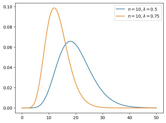
A random variable \(W\) on \(\RR_+\) is said to have the Erlang distribution if its density has the form
for some \(n \in \NN\) and \(\lambda > 0\).
The parameters \(n\) and \(\lambda\) are called the shape and rate parameters respectively.
The next figure shows the shape for two parameterizations.
The CDF of the Erlang distribution is
The Erlang distribution is of interest to us because of the following fact.
Lemma 1.1 (Distribution of Sum of Exponentials)
If, for some \(\lambda > 0\), the sequence \((W_i)\) is IID and exponentially distributed with rate \(\lambda\), then \(J_n := \sum_{i=1}^n W_i\) has the Erlang distribution with shape \(n\) and rate \(\lambda\).
This connects to Poisson process theory, as we shall soon see.
1.5. Exercises#
Exercise 1.1
Due to its memoryless property, we can “stop” and “restart” an exponential draw without changing its distribution.
To illustrate this, we can think of fixing \(\lambda > 0\), drawing from \(\Exp(\lambda)\), and stopping and restarting whenever a threshold \(s\) is crossed.
In particular, consider the random variable \(X\) defined as follows:
Draw \(Y\) from \(\Exp(\lambda)\).
If \(Y \leq s\), set \(X = Y\).
If not, draw \(Z\) independently from \(\Exp(\lambda)\) and set \(X = s + Z\).
Show that \(X \sim \Exp(\lambda)\).
Solution
Let \(X\) be constructed as in the statement of the exercise and fix \(t > 0\).
Notice that \(X > s + t\) if and only if \(Y > s\) and \(Z > t\).
As a result of this fact and independence,
At the same time, \(X > s-t\) if and only if \(Y > s-t\), so
Either way, we have \(X \sim \Exp(\lambda)\), as was to be shown.
Exercise 1.2
Fix \(\lambda = 0.5\) and \(s=1.0\).
Simulate 1,000 draws of \(X\) using the algorithm above.
Plot the fraction of the sample exceeding \(t\) for each \(t \geq 0\) (on a grid) and compare to \(t \mapsto e^{-\lambda t}\).
Is the fit good? How about if the number of draws is increased?
Are the results in line with those of the previous exercise?
Solution
Here’s one solution, starting with 1,000 draws.
λ = 0.5
np.random.seed(1234)
t_grid = np.linspace(0, 10, 200)
@njit
def draw_X(s=1.0, n=1_000):
draws = np.empty(n)
for i in range(n):
Y = np.random.exponential(scale=1/λ)
if Y <= s:
X = Y
else:
Z = np.random.exponential(scale=1/λ)
X = s + Z
draws[i] = X
return draws
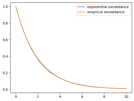
fig, ax = plt.subplots()
draws = draw_X()
empirical_exceedance = [np.mean(draws > t) for t in t_grid]
ax.plot(t_grid, np.exp(- λ * t_grid), label='exponential exceedance')
ax.plot(t_grid, empirical_exceedance, label='empirical exceedance')
ax.legend()
plt.show()
The fit is already very close, which matches with the theory in .
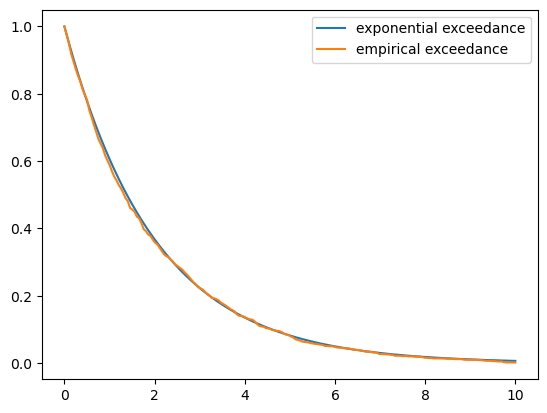
The two lines become indistinguishable as \(n\) is increased further.
fig, ax = plt.subplots()
draws = draw_X(n=10_000)
empirical_exceedance = [np.mean(draws > t) for t in t_grid]
ax.plot(t_grid, np.exp(- λ * t_grid), label='exponential exceedance')
ax.plot(t_grid, empirical_exceedance, label='empirical exceedance')
ax.legend()
plt.show()