2. Poisson Processes#
In addition to what’s in Anaconda, this lecture will need the following libraries:
!pip install quantecon
2.1. Overview#
Counting processes count the number of “arrivals” occurring by a given time (e.g., the number of visitors to a website, the number of customers arriving at a restaurant, etc.)
Counting processes become Poisson processes when the time interval between arrivals is IID and exponentially distributed.
Exponential distributions and Poisson processes have deep connections to continuous time Markov chains.
For example, Poisson processes are one of the simplest nontrivial examples of a continuous time Markov chain.
In addition, when continuous time Markov chains jump between states, the time between jumps is necessarily exponentially distributed.
In discussing Poisson processes, we will use the following imports:
import numpy as np
import matplotlib.pyplot as plt
import quantecon as qe
from numba import njit
from scipy.special import factorial, binom
2.2. Counting Processes#
Let’s start with the general case of an arbitrary counting process.
2.2.1. Jumps and Counts#
Let \((J_k)\) be an increasing sequence of nonnegative random variables satisfying \(J_k \to \infty\) with probability one.
For example, \(J_k\) might be the time the \(k\)-th customer arrives at a shop.
Then
is the number of customers that have visited by time \(t\).
The next figure illustrate the definition of \(N_t\) for a given jump sequence \(\{J_k\}\).
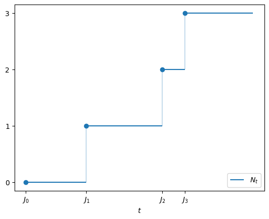
An alternative but equivalent definition is
As a function of \(t\), the process \(N_t\) is called a counting process.
The jump times \((J_k)\) are sometimes called arrival times and the intervals \(J_k - J_{k-1}\) are called wait times or holding times.
2.2.2. Exponential Holding Times#
A Poisson process is a counting process with independent exponential holding times.
In particular, suppose that the arrival times are given by \(J_0 = 0\) and
where \((W_i)\) are IID exponential with some fixed rate \(\lambda\).
Then the associated counting process \((N_t)\) is called a Poisson process with rate \(\lambda\).
The rationale behind the name is that, for each \(t > 0\), the random variable \(N_t\) has the Poisson distribution with parameter \(t \lambda\).
In other words,
For example, since \(N_t = 0\) if and only if \(W_1 > t\), we have
and the right hand side agrees with (2.2) when \(k=0\).
This sets up a proof by induction, which is time consuming but not difficult — the details can be found in \(\S29\) of [Howard, 2017].
Another way to show that \(N_t\) is Poisson with rate \(\lambda\) is to appeal to Lemma 1.1.
We observe that
Inserting the expression for the Erlang CDF in (1.5) with shape \(n+1\) and rate \(\lambda\), we obtain
This is the (integer valued) CDF for the Poisson distribution with parameter \(t \lambda\).
An exercise at the end of the lecture asks you to verify that \(N_t\) is Poisson-\((t \lambda )\) informally via simulation.
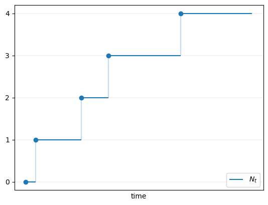
The next figure shows one realization of a Poisson process \((N_t)\), with jumps at each new arrival.
2.3. Stationary Independent Increments#
One of the defining features of a Poisson process is that it has stationary and independent increments.
This is due to the memoryless property of exponentials.
It means that
the variables \(\{N_{t_{i+1}} - N_{t_i}\}_{i \in I}\) are independent for any strictly increasing finite sequence \((t_i)_{i \in I}\) and
the distribution of \(N_{t+h} - N_t\) depends on \(h\) but not \(t\).
A detailed proof can be found in Theorem 2.4.3 of [Norris, 1998].
Instead of repeating this, we provide some intuition from a discrete approximation.
In the discussion below, we use the following well known fact: If \((\theta_n)\) is a sequence such that \(n \theta_n\) converges, then
(The exercises ask you to examine this claim visually.)
We now return to the environment where we linked the geometric distribution to the exponential.
That is, we fix small \(h > 0\) and let \(t_i := ih\) for all \(i \in \ZZ_+\).
Let \((V_i)\) be IID binary random variables with \(\PP\{V_i = 1\} = h \lambda\) for some \(\lambda > 0\).
Linking to our previous discussion,
either one or zero customers visits a shop at each \(t_i\).
\(V_i = 1\) means that a customer visits at time \(t_i\).
Visits occur with probability \(h \lambda\), which is proportional to the length of the interval between grid points.
We learned that the wait time until the first visit is approximately exponential with rate \(t \lambda\).
Since \((V_i)\) is IID, the same is true for the second wait time and so on.
Moreover, these wait times are independent, since they depend on separate subsets of \((V_i)\).
Let \(\hat N_t\) count the number of visits by time \(t\), as shown in the next figure.
(\(V_i = 1\) is indicated by a vertical line at \(t_i = i h\).)
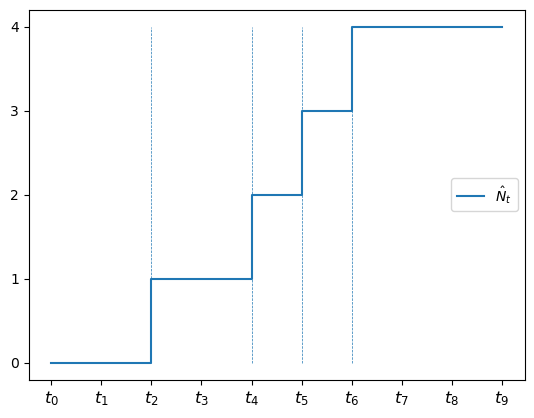
We expect from the discussion above that \((\hat N_t)\) approximates a Poisson process.
This intuition is correct because, fixing \(t\), letting \(k := \max\{i \in \ZZ_+ \,:\, t_i \leq t\}\) and applying (2.3), we have
Using the fact that \(kh = t_k \approx t\) as \(h \to 0\), we see that \(\hat N_t\) is approximately Poisson with rate \(t \lambda\), just as we expected.
This approximate construction of a Poisson process helps illustrate the property of stationary independent increments.
For example, if we fix \(s, t\), then \(\hat N_{s + t} - \hat N_s\) is the number of visits between \(s\) and \(s+t\), so that
Suppose there are \(k\) grid points between \(s\) and \(s+t\), so that \(t \approx kh\).
Then
This illustrates the idea that, for a Poisson process \((N_t)\), we have
In particular, increments are stationary (the distribution depends on \(t\) but not \(s\)).
The approximation also illustrates independence of increments, since, in the approximation, increments depend on separate subsets of \((V_i)\).
2.4. Uniqueness#
What other counting processes have stationary independent increments?
Remarkably, the answer is none:
Theorem 2.1 (Characterization of Poisson Processes)
If \((M_t)\) is a stochastic process supported on \(\ZZ_+\) and starting at 0 with the property that its increments are stationary and independent, then \((M_t)\) is a Poisson process.
In particular, there exists a \(\lambda > 0\) such that
for any \(s, t\).
The proof is similar to our earlier proof that the exponential distribution is the only memoryless distribution.
Details can be found in Section 6.2 of [Pardoux, 2008] or Theorem 2.4.3 of [Norris, 1998].
2.4.1. The Restarting Property#
An important consequence of stationary independent increments is the restarting property, which means that, when simulating, we can freely stop and restart a Poisson process at any time:
Theorem 2.2 (Poisson Processes can be Paused and Restarted)
If \((N_t)\) is a Poisson process, \(s > 0\) and \((M_t)\) is defined by \(M_t = N_{s+t} - N_s\) for \(t \geq 0\), then \((M_t)\) is a Poisson process independent of \((N_r)_{r \leq s}\).
Proof. Independence of \((M_t)\) and \((N_r)_{r \leq s}\) follows from indepenence of the increments of \((N_t)\).
In view of the uniqueness statement above, we can verify that \((M_t)\) is a Poisson process by showing that \((M_t)\) starts at zero, takes values in \(\ZZ_+\) and has stationary independent increments.
It is clear that \((M_t)\) starts at zero and takes values in \(\ZZ_+\).
In addition, if we take any \(t < t'\), then
Hence \((M_t)\) has stationary increments and, using the relation \(M_{t'} - M_t = N_{s+t'} - N_{s + t}\) again, the increments are independent as well.
We conclude that \((N_{s+t} - N_s)_{t \geq 0}\) is indeed a Poisson process independent of \((N_r)_{r \leq s}\).
2.5. Exercises#
Exercise 2.1
Fix \(\lambda > 0\) and draw \(\{W_i\}\) as IID exponentials with rate \(\lambda\).
Set \(J_n := W_1 + \cdots W_n\) with \(J_0 = 0\) and \(N_t := \sum_{n \geq 0} n \mathbb 1\{ J_n \leq t < J_{n+1} \}\).
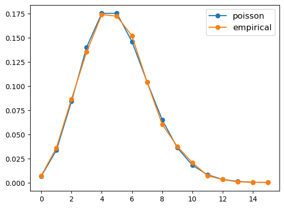
Provide a visual test of the claim that \(N_t\) is Poisson with parameter \(t \lambda\).
Do this by fixing \(t = T\), generating many independent draws of \(N_T\) and comparing the empirical distribution of the sample with a Poisson distribution with rate \(T \lambda\).
Try first with \(\lambda = 0.5\) and \(T=10\).
Solution
Here is one solution.
The figure shows that the fit is already good with a modest sample size.
Increasing the sample size will further improve the fit.
λ = 0.5
T = 10

def poisson(k, r):
    "Poisson pmf with rate r."
    return np.exp(-r) * (r**k) / factorial(k)

@njit
def draw_Nt(max_iter=1e5):
    J = 0
    n = 0
    while n < max_iter:
        W = np.random.exponential(scale=1/λ)
        J += W
        if J > T:
            return n
        n += 1

@njit
def draw_Nt_sample(num_draws):
    draws = np.empty(num_draws)
    for i in range(num_draws):
        draws[i] = draw_Nt()
    return draws


sample_size = 10_000
sample = draw_Nt_sample(sample_size)
max_val = sample.max()
vals = np.arange(0, max_val+1)

fig, ax = plt.subplots()

ax.plot(vals, [poisson(v, T * λ) for v in vals],
    marker='o', label='poisson')
ax.plot(vals, [np.mean(sample==v) for v in vals],
    marker='o', label='empirical')

ax.legend(fontsize=12)
plt.show()
Exercise 2.2
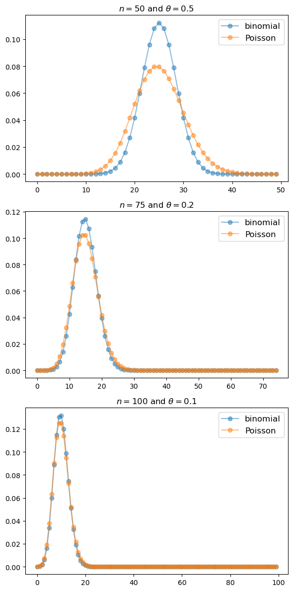
In the lecture we used the fact that \(\Binomial(n, \theta) \approx \Poisson(n \theta)\) when \(n\) is large and \(\theta\) is small.
Investigate this relationship by plotting the distributions side by side.
Experiment with different values of \(n\) and \(\theta\).
Solution
Here is one solution. It shows that the approximation is good when \(n\) is large and \(\theta\) is small.
def binomial(k, n, p):
    # Binomial(n, p) pmf evaluated at k
    return binom(n, k) * p**k * (1-p)**(n-k)

θ_vals = 0.5, 0.2, 0.1

n_vals = 50, 75, 100

fig, axes = plt.subplots(len(n_vals), 1, figsize=(6, 12))

for n, θ, ax in zip(n_vals, θ_vals, axes.flatten()):

    k_grid = np.arange(n)
    binom_vals = [binomial(k, n, θ) for k in k_grid]
    poisson_vals = [poisson(k, n * θ) for k in k_grid]
    ax.plot(k_grid, binom_vals, 'o-', alpha=0.5, label='binomial')
    ax.plot(k_grid, poisson_vals, 'o-', alpha=0.5, label='Poisson')
    ax.set_title(f'$n={n}$ and $\\theta = {θ}$')
    ax.legend(fontsize=12)

fig.tight_layout()
plt.show()