5. The Kolmogorov Forward Equation#
In addition to what’s in Anaconda, this lecture will need the following libraries:
!pip install quantecon
5.1. Overview#
In this lecture we approach continuous time Markov chains from a more analytical perspective.
The emphasis will be on describing distribution flows through vector-valued differential equations and their solutions.
These distribution flows show how the time \(t\) distribution associated with a given Markov chain \((X_t)\) changes over time.
Distribution flows will be identified with initial value problems generated by autonomous linear ordinary differential equations (ODEs) in vector space.
We will see that the solutions of these flows are described by Markov semigroups.
This leads us back to the theory we have already constructed – some care will be taken to clarify all the connections.
In order to avoid being distracted by technicalities, we continue to defer our treatment of infinite state spaces, assuming throughout this lecture that \(|S| = n\).
As before, \(\dD\) is the set of all distributions on \(S\).
We will use the following imports
import numpy as np
import scipy as sp
import matplotlib.pyplot as plt
import quantecon as qe
from numba import njit
from scipy.linalg import expm

from matplotlib import cm
from mpl_toolkits.mplot3d import Axes3D
from mpl_toolkits.mplot3d.art3d import Poly3DCollection
5.2. From Difference Equations to ODEs#
Previously we generated this figure, which shows how distributions evolve over time for the inventory model under a certain parameterization:
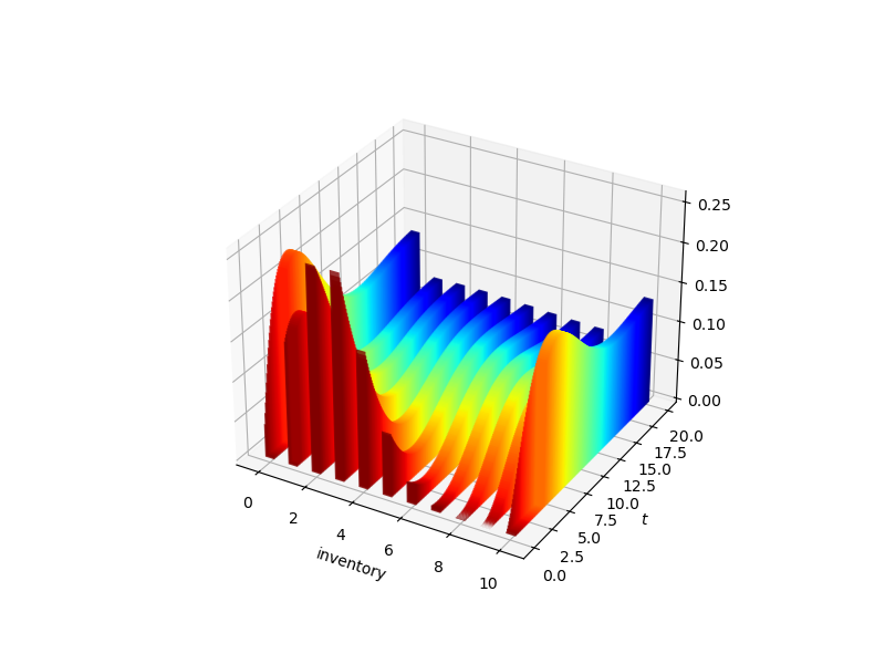
Fig. 5.1 Probability flows for the inventory model.#
(Hot colors indicate early dates and cool colors denote later dates.)
We also learned how this flow is related to the Kolmogorov backward equation, which is an ODE.
In this section we examine distribution flows and their connection to ODEs and continuous time Markov chains more systematically.
5.2.1. Review of the Discrete Time Case#
Let \((X_t)\) be a discrete time Markov chain with Markov matrix \(P\).
Recall that, in the discrete time case, the distribution \(\psi_t\) of \(X_t\) updates according to
where distributions are understood as row vectors.
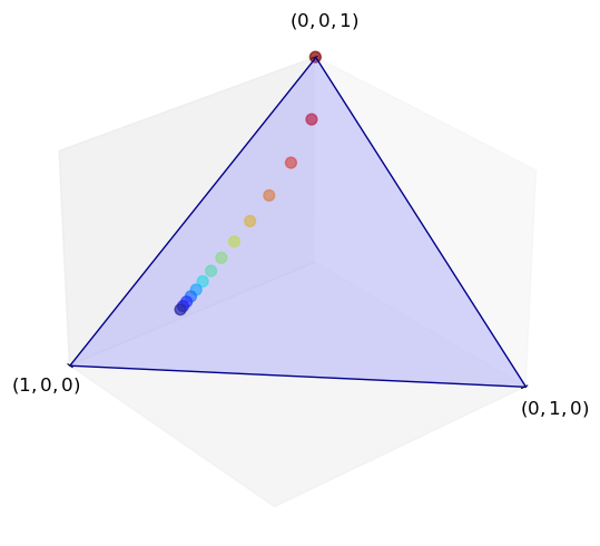
Here’s a visualization for the case \(S = \{0, 1, 2\}\), so that \(\dD\) is the standard simplex in \(\RR^3\).
The initial condition is (0, 0, 1) and the Markov matrix is
P = ((0.9, 0.1, 0.0),
     (0.4, 0.4, 0.2),
     (0.1, 0.1, 0.8))
There’s a sense in which a discrete time Markov chain “is” a homogeneous linear difference equation in distribution space.
To clarify this, suppose we take \(G\) to be a linear map from \(\dD\) to itself and write down the difference equation
Because \(G\) is a linear map from a finite dimensional space to itself, it can be represented by a matrix.
Moreover, a matrix \(P\) is a Markov matrix if and only if \(\psi \mapsto \psi P\) sends \(\dD\) into itself (check it if you haven’t already).
So, under the stated conditions, our difference equation (5.1) uniquely identifies a Markov matrix, along with an initial condition \(\psi_0\).
Together, these objects identify the joint distribution of a discrete time Markov chain, as previously described.
5.2.2. Shifting to Continuous Time#
We have just argued that a discrete time Markov chain can be identified with a linear difference equation evolving in \(\dD\).
This strongly suggests that a continuous time Markov chain can be identified with a linear ODE evolving in \(\dD\).
This intuition is correct and important.
The rest of the lecture maps out the main ideas.
5.3. ODEs in Distribution Space#
Consider linear differential equation given by
where
\(Q\) is an \(n \times n\) matrix,
distributions are again understood as row vectors, and
derivatives are taken element by element, so that
5.3.1. Solutions to Linear Vector ODEs#
Using the matrix exponential, the unique solution to the initial value problem (5.2) is
To check that (5.3) is a solution, we use (4.7) again to get
The first equality can be written as \(P_t' = Q P_t\) and this is just the Kolmogorov backward equation.
The second equality can be written as
and is called the Kolmogorov forward equation.
Applying the Kolmogorov forward equation, we obtain
This confirms that (5.3) solves (5.2).
Here’s an example of three distribution flows with dynamics generated by (5.2), one starting from each vertex.
The code uses (5.3) with matrix \(Q\) given by
Q = ((-3, 2, 1),
     (3, -5, 2),
     (4, 6, -10))
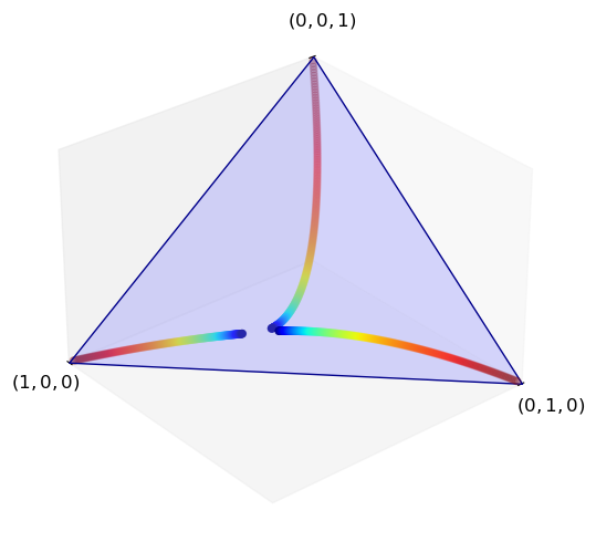
(Distributions cool over time, so initial conditions are hot colors.)
5.3.2. Forwards vs Backwards Equations#
As the above discussion shows, we can take the Kolmogorov forward equation \(P_t' = P_t Q\) and premultiply by any distribution \(\psi_0\) to get the distribution ODE \(\psi'_t = \psi_t Q\).
In this sense, we can understand the Kolmogorov forward equation as pushing distributions forward in time.
Analogously, we can take the Kolmogorov backward equation \(P_t' = Q P_t\) and postmultiply by any vector \(h\) to get
Recalling that \((P_t h)(x) = \EE [ h(X_t) \,|\, X_0 = x]\), this vector ODE tells us how expectations evolve, conditioning backward to time zero.
Both the forward and the backward equations uniquely pin down the same solution \(P_t = e^{tQ}\) when combined with the initial condition \(P_0 = I\).
5.3.3. Matrix- vs Vector-Valued ODEs#
The ODE \(\psi'_t = \psi_t Q\) is sometimes called the Fokker–Planck equation (although this terminology is most commonly used in the context of diffusions).
It is a vector-valued ODE that describes the evolution of a particular distribution path.
By comparison, the Kolmogorov forward equation is (like the backward equation) a differential equation in matrices.
(And matrices are really maps, which send vectors into vectors.)
Operating at this level is less intuitive and more abstract than working with the Fokker–Planck equation.
But, in the end, the object that we want to describe is a Markov semigroup.
The Kolmogorov forward and backward equations are the ODEs that define this fundamental object.
5.3.4. Preserving Distributions#
In the simulation above, \(Q\) was chosen with some care, so that the flow remains in \(\dD\).
What are the exact properties we require on \(Q\) such that \(\psi_t\) is always in \(\dD\)?
This is an important question, because we are setting up an exact correspondence between linear ODEs that evolve in \(\dD\) and continuous time Markov chains.
Recall that the linear update rule \(\psi \mapsto \psi P\) is invariant on \(\dD\) if and only if \(P\) is a Markov matrix.
So now we can rephrase our key question regarding invariance on \(\dD\):
What properties do we need to impose on \(Q\) so that \(P_t = e^{tQ}\) is a Markov matrix for all \(t\)?
A square matrix \(Q\) is called an intensity matrix if \(Q\) has zero row sums and \(Q(x, y) \geq 0\) whenever \(x \not= y\).
Theorem 5.1
If \(Q\) is a matrix on \(S\) and \(P_t := e^{tQ}\), then the following statements are equivalent:
\(P_t\) is a Markov matrix for all \(t\).
\(Q\) is an intensity matrix.
The proof is related to that of Lemma 4.2 and is found as a solved exercise below.
Corollary 5.1
If \(Q\) is an intensity matrix on finite \(S\) and \(P_t = e^{tQ}\) for all \(t \geq 0\), then \((P_t)\) is a Markov semigroup.
We call \((P_t)\) the Markov semigroup generated by \(Q\).
Later we will see that this result extends to the case \(|S| = \infty\) under some mild restrictions on \(Q\).
5.4. Jump Chains#
Let’s return to the chain \((X_t)\) created from jump chain pair \((\lambda, K)\) in Algorithm 4.1.
We found that the semigroup is given by
Using the fact that \(K\) is a Markov matrix and the jump rate function \(\lambda\) is nonnegative, you can easily check that \(Q\) satisfies the definition of an intensity matrix.
Hence \((P_t)\), the Markov semigroup for the jump chain \((X_t)\), is the semigroup generated by the intensity matrix \(Q(x, y) = \lambda(x) (K(x, y) - I(x, y))\).
We can differentiate \(P_t = e^{tQ}\) to obtain the Kolmogorov forward equation \(P_t' = P_t Q\).
We can then premultiply by \(\psi_0 \in \dD\) to get \(\psi_t' = \psi_t Q\), which is the Fokker–Planck equation.
More explicitly, for given \(y \in S\),
The rate of probability flow into \(y\) is equal to the inflow from other states minus the outflow.
5.5. Summary#
We have seen that any intensity matrix \(Q\) on \(S\) defines a Markov semigroup via \(P_t = e^{tQ}\).
Henceforth, we will say that \((X_t)\) is a Markov chain with intensity matrix \(Q\) if \((X_t)\) is a Markov chain with Markov semigroup \((e^{tQ})\).
While our discussion has been in the context of a finite state space, later we will see that these ideas carry over to an infinite state setting under mild restrictions.
We have also hinted at the fact that every continuous time Markov chain is a Markov chain with intensity matrix \(Q\) for some suitably chosen \(Q\).
Later we will prove this to be universally true when \(S\) is finite and true under mild conditions when \(S\) is countably infinite.
Intensity matrices are important because
they are the natural infinitesimal descriptions of Markov semigroups,
they are often easy to write down in applications and
they provide an intuitive description of dynamics.
Later, we will see that, for a given intensity matrix \(Q\), the elements are understood as follows:
when \(x \not= y\), the value \(Q(x, y)\) is the “rate of leaving \(x\) for \(y\)” and
\(-Q(x, x) \geq 0\) is the “rate of leaving \(x\)” .
5.6. Exercises#
Exercise 5.1
Let \((P_t)\) be a Markov semigroup such that \(t \mapsto P_t(x, y)\) is differentiable at all \(t \geq 0\) and \((x, y) \in S \times S\).
(The derivative at \(t=0\) is the usual right derivative.)
Define (pointwise, at each \((x,y)\)),
Assuming that this limit exists, and hence \(Q\) is well-defined, show that
both hold. (These are the Kolmogorov forward and backward equations.)
Solution
Let \((P_t)\) be a Markov semigroup and let \(Q\) be as defined in the statement of the exercise.
Fix \(t \geq 0\) and \(h > 0\).
Combining the semigroup property and linearity with the restriction \(P_0 = I\), we get
Taking \(h \downarrow 0\) and using the definition of \(Q\) give \(P_t' = P_t Q\), which is the Kolmogorov forward equation.
For the backward equation we observe that
also holds. Taking \(h \downarrow 0\) gives the Kolmogorov backward equation.
Exercise 5.2
Recall our model of jump chains with state-dependent jump intensities given by rate function \(x \mapsto \lambda(x)\).
After a wait time with exponential rate \(\lambda(x) \in (0, \infty)\), the state transitions from \(x\) to \(y\) with probability \(K(x,y)\).
We found that the associated semigroup \((P_t)\) satisfies the Kolmogorov backward equation \(P'_t = Q P_t\) with
Show that \(Q\) is an intensity matrix and that (5.4) holds.
Solution
Let \(Q\) be as defined in (5.5).
We need to show that \(Q\) is nonnegative off the diagonal and has zero row sums.
The first assertion is immediate from nonnegativity of \(K\) and \(\lambda\).
For the second, we use the fact that \(K\) is a Markov matrix, so that, with \(1\) as a column vector of ones,
Exercise 5.3
Prove Theorem 5.1 by adapting the arguments in Lemma 4.2. (This is nontrivial but worth at least trying.)
Hint: The constant \(m\) in the proof can be set to \(\max_x |Q(x, x)|\).
Solution
Suppose that \(Q\) is an intensity matrix, fix \(t \geq 0\) and set \(P_t = e^{tQ}\).
The proof from Lemma 4.2 that \(P_t\) has unit row sums applies directly to the current case.
The proof of nonnegativity of \(P_t\) can be applied after some modifications.
To this end, set \(m := \max_x |Q(x,x)|\) and \(\hat P := I + Q / m\).
You can check that \(\hat P\) is a Markov matrix and that \(Q = m( \hat P - I)\).
The rest of the proof of nonnegativity of \(P_t\) is unchanged and we will not repeat it.
We conclude that \(P_t\) is a Markov matrix.
Regarding the converse implication, suppose that \(P_t = e^{tQ}\) is a Markov matrix for all \(t\) and let \(1\) be a column vector of ones.
Because \(P_t\) has unit row sums and differentiation is linear, we can employ the Kolmogorov backward equation to obtain
Hence \(Q\) has zero row sums.
We can use the definition of the matrix exponential to obtain, for any \(x, y\) and \(t \geq 0\),
From this equality and the assumption that \(P_t\) is a Markov matrix for all \(t\), we see that the off diagonal elements of \(Q\) must be nonnegative.
Hence \(Q\) is an intensity matrix.